1c. Visualising models

The following tutorial will demonstrate how to use the Loop structural visualisation module. This module provides a wrapper for the lavavu model that is written by Owen Kaluza.

Lavavu allows for interactive visualisation of 3D models within a jupyter notebook environment.

Imports

Import the required objects from LoopStructural for visualisation and model building

from LoopStructural import GeologicalModel
from LoopStructural.visualisation import Loop3DView

from LoopStructural.datasets import load_claudius  # demo data

Build the model

data, bb = load_claudius()
model = GeologicalModel(bb[0, :], bb[1, :])
model.set_model_data(data)
strati = model.create_and_add_foliation("strati",nelements=1e4)
vals = [0, 60, 250, 330, 600]
for i in range(len(vals) - 1):
    model.stratigraphic_column.add_unit(
        f"unit_{i}",
        thickness=vals[i + 1] - vals[i],
        id=i,
    )
model.stratigraphic_column.group_mapping['Group_0'] = 'strati'

Visualising results

The Loop3DView is an LoopStructural class that provides easy 3D plotting options for plotting data points and resulting implicit functions.

the Loop3DView is a wrapper around the pyvista Plotter class. Allowing any of the methods for the pyvista Plotter class to be used.

The implicit function can be visualised by looking at isosurfaces of the scalar field.

viewer = Loop3DView()
viewer.plot_surface(feature,**kwargs)

Where optional kwargs can be:

• value specifying the number of regularly spaced isosurfaces

• paint_with the geological feature to colour the surface with

• cmap colour map for the colouring

• normals to plot the normal vectors to the surface

• name to give the surface

• colour the colour of the surface

• opacity the opacity of the surface

• vmin minimum value of the colour map

• vmax maximum value of the colour map

• pyvista_kwargs - other kwargs for passing directly to pyvista Plotter.add_mesh

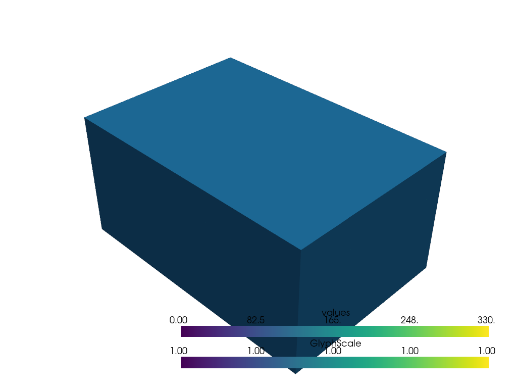
Alternatively the scalar fields can be displayed on a rectangular cuboid.

viewer.plot_scalar_field(geological_feature, **kwargs)

Other possible kwargs are:

• cmap colour map for the property

• vmin minimum value of the colour map

• vmax maximum value of the colour map

• opacity the opacity of the block

• pyvista_kwargs - other kwargs for passing directly to pyvista Plotter.add_mesh

The input data for the model can be visualised by calling either:

viewer.plot_data(feature,**kwargs)

Where optional kwargs can be: - value - whether to add value data - vector - whether to add gradient data - scale - scale of the gradient vectors - pyvista_kwargs - other kwargs for passing directly to pyvista Plotter.add_mesh

The gradient of a geological feature can be visualised by calling:

viewer.add_vector_field(feature, **kwargs)

Where the optional kwargs can be: - scale - scale of the gradient vectors

viewer = Loop3DView(model, background="white")

# determine the number of unique surfaces in the model from
# the input data and then calculate isosurfaces for this

viewer.plot_surface(strati, value=vals, cmap="prism", paint_with=strati)
viewer.display()
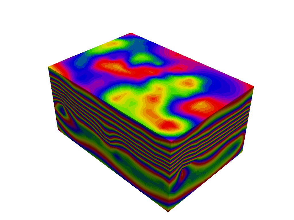
viewer = Loop3DView(model, background="white")

viewer.plot_scalar_field(strati, cmap="prism")
viewer.display()
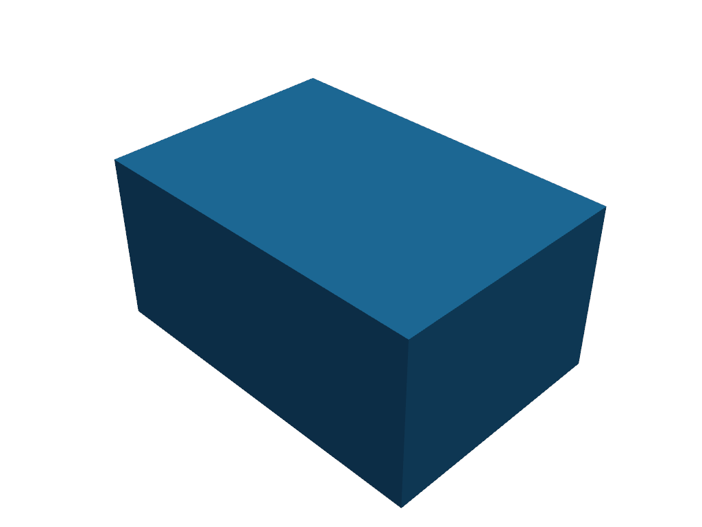
viewer = Loop3DView(model, background="white")
# print(viewer._build_stratigraphic_cmap(model))
viewer.plot_block_model(cmap='tab20')
viewer.display()
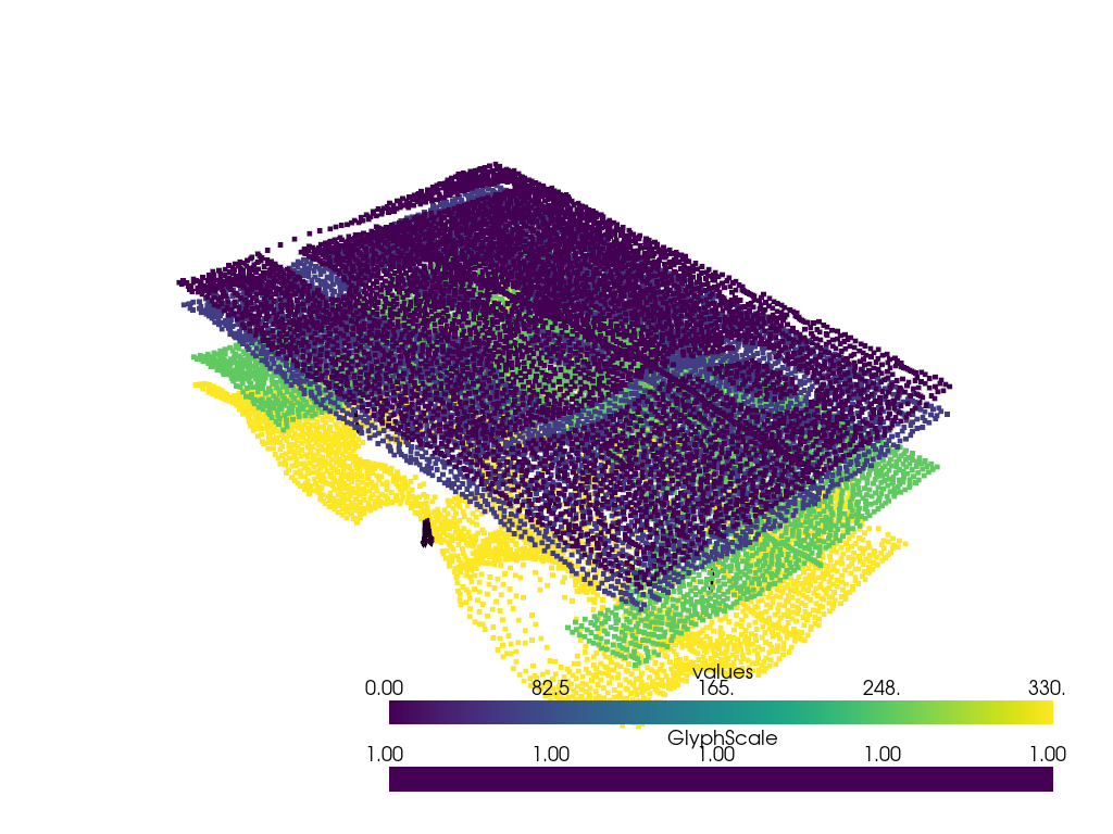
viewer = Loop3DView(model, background="white")

# Add the data addgrad/addvalue arguments are optional
viewer.plot_data(strati, vector=True, value=True)
viewer.display()  # to add an interactive display

• 
• 
• 
•