1b. Implicit surface modelling

This tutorial will demonstrate how to create an implicit surface representation of surfaces from a combination of orientation and location observations.

Implicit surface representation involves finding an unknown function where \(f(x,y,z)\) matches observations of the surface geometry. We generate a scalar field where the scalar value is the distance away from a reference horizon. The reference horizon is arbritary and can either be:

• a single geological surface where the scalar field would represent the signed distance away from this surface. (above the surface positive and below negative)

• Where multiple conformable horizons are observed the same scalar field can be used to represent these surfaces and the thickness of the layers is used to determine the relative scalar value for each surface

This tutorial will demonstrate both of these approaches for modelling a number of horizons picked from seismic data sets, by following the next steps: 1. Creation of a geological model, which includes: * Presentation and visualization of the data * Addition of a geological feature, which in this case is the stratigraphy of the model. 2. Visualization of the scalar field.

Imports

Import the required objects from LoopStructural for visualisation and model building

from LoopStructural import GeologicalModel
from LoopStructural.visualisation import Loop3DView
from LoopStructural.datasets import load_claudius  # demo data

import numpy as np

Load Example Data

The data for this example can be imported from the example datasets module in LoopStructural. The load_claudius function provides both the data and the bounding box (bb) for the model.

data, bb = load_claudius()

# Display unique scalar field values in the dataset
print(data["val"].unique())

[250. 330.   0.  60.  nan]

Create Geological Model

Define the model area using the bounding box (bb) and create a GeologicalModel instance.

model = GeologicalModel(bb[0, :], bb[1, :])

Link Data to Geological Model

A pandas dataframe with appropriate columns is used to link the data to the geological model. Key columns include: * X, Y, Z: Coordinates of the observation * feature_name: Name linking the data to a model object * val: Scalar field value representing distance from a reference horizon * nx, ny, nz: Components of the normal vector to the surface gradient * strike, dip: Strike and dip angles

# Display unique feature names in the dataset
print(data["feature_name"].unique())

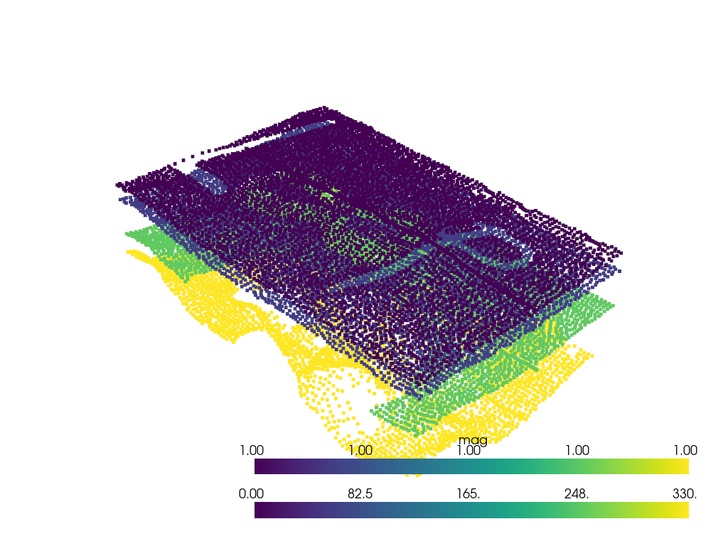
# Visualize the data points and orientation vectors in 3D
viewer = Loop3DView(background="white")
viewer.add_points(
    data[~np.isnan(data["val"])][["X", "Y", "Z"]].values,
    scalars=data[~np.isnan(data["val"])]["val"].values,
)
viewer.add_arrows(
    data[~np.isnan(data["nx"])][["X", "Y", "Z"]].values,
    direction=data[~np.isnan(data["nx"])][["nx", "ny", "nz"]].values,
)
viewer.display()

# Link the data to the geological model
model.set_model_data(data)

['strati']

Add Geological Features

The GeologicalModel can include various geological features such as foliations, faults, unconformities, and folds. In this example, we add a foliation using the create_and_add_foliation method.

# Define stratigraphic column with scalar field ranges for each unit
vals = [0, 60, 250, 330, 600]
strat_column = {"strati": {}}
for i in range(len(vals) - 1):
    strat_column["strati"]["unit_{}".format(i)] = {
        "min": vals[i],
        "max": vals[i + 1],
        "id": i,
    }

# Set the stratigraphic column in the model
model.set_stratigraphic_column(strat_column)

# Add a foliation to the model
strati = model.create_and_add_foliation(
    "strati",
    interpolatortype="FDI",  # Finite Difference Interpolator
    nelements=int(1e4),  # Number of elements for discretization
    buffer=0.3,  # Buffer percentage around the model area
    damp=True,  # Add damping for stability
)

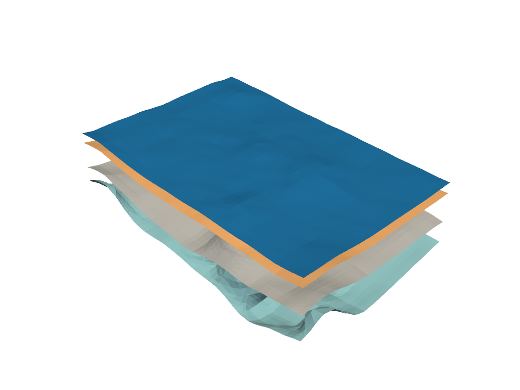
Visualize Model Surfaces

Plot the surfaces of the geological model using a 3D viewer.

print(model.stratigraphic_column.to_dict())
viewer = Loop3DView(model)
viewer.plot_model_surfaces(cmap="tab20")
viewer.display()

{'elements': [{'name': 'Basement', 'colour': 'grey', 'thickness': inf, 'uuid': 'ff775f6a-43bc-4d88-9ee7-bc593886d40b', 'id': 0}, {'uuid': '6a038684-d9b8-468b-b717-5b4e38449e3f', 'name': 'Base Unconformity', 'unconformity_type': 'erode'}, {'name': 'Basement', 'colour': 'grey', 'thickness': inf, 'uuid': 'e2ad68e5-cb0b-4dd5-9a15-e9c07ce3080b', 'id': 1}, {'uuid': '33885860-e638-4d2e-99e2-0457f0e2b764', 'name': 'Base Unconformity', 'unconformity_type': 'erode'}, {'name': 'unit_0', 'colour': [0.5533612487413869, 0.4085212463020087, 0.1456926068266835], 'thickness': 60, 'uuid': 'ffb08303-fcd6-46b1-9edb-b03c46623f10', 'id': 2}, {'name': 'unit_1', 'colour': [0.43276802613334087, 0.7184937550895265, 0.09245407710991571], 'thickness': 190, 'uuid': '905e9d51-91ef-4850-ab15-dd17a499880e', 'id': 3}, {'name': 'unit_2', 'colour': [0.5345311883953344, 0.13992637896814641, 0.37448325806124017], 'thickness': 80, 'uuid': '04809369-e7d1-4195-b4ad-bdd1e76b6d54', 'id': 4}, {'name': 'unit_3', 'colour': [0.5375750687846683, 0.049827761127233305, 0.5386750980520866], 'thickness': 270, 'uuid': '30dfea56-e454-4100-811f-a0c2a117c63e', 'id': 5}, {'uuid': 'a8ad4d02-00bd-4a48-bcbb-929fc05d9f69', 'name': 'stratiunconformity', 'unconformity_type': 'erode'}]}

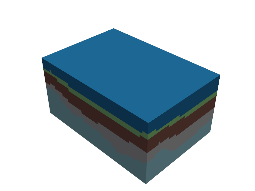
Visualize Block Diagram

Plot a block diagram of the geological model to visualize the stratigraphic units in 3D.

viewer = Loop3DView(model)
viewer.plot_block_model(cmap="tab20")
viewer.display()