Note
Go to the end to download the full example code.
1a. Getting started#
This tutorial will demonstrate how to setup a basic geological model for using with LoopStructural.
Implicit surface modelling#
LoopStructural uses implicit surface representation to build upper and lower surfaces for geological horizons. Implicit surface representation involves approximating an unknown function \(f(x,y,z)\) where the function value represents the distance from a reference horizon. Geological surfaces can be represented by tracing isovalues of the scalar field. The implicit function is approximated using numerical techniques to find a function that fits the observations. There are two main approaches used in implicit modelling for approximating these implicit functions:
Data supported approximation using polynomial trend methods
Discrete approaches using a interpolation support and minimising the misfit to observations and a regularisation term.
The main interpolation approach used by LoopStructural is Discrete implicit modelling approaches where the geological observations are combined with a regularisation term to find the best resulting surface.
There are two main interpolators that can be used:
Piecewise Linear interpolator - which uses a regular tetrahedron mesh with P1 finite elements
Finite difference interpolator - which uses a regular Cartesian grid with cubic elements using trilinear interpolation
Data types#
There are three constraints that can be added to the interpolator
Value constraints which set enforce \(f(x,y,z) = value\)
Gradient constraints which set the interpolated gradient of the function to be orthogonal to an observed vector \(f'(x,y,z) \cdot v = 0\)
Gradient norm constraints which set the partial derivative of the implicit function to be equal to the components of the observed normal vector.
GeologicalFeatures#
A typical geological model may contain multiple geological interfaces, including unconformities and faults. Conformable surfaces can be represented by a single implicit function where different isosurfaces represent different horizons.
In LoopStructural an implicit function is encapsulated by a GeologicalFeature. The GeologicalFeature represents an object within the model that can be evaluated at any location within the model area.
Define the model area Origin = (0,0,0) Maximum = (10,10,10)
Create a pointset representing two flat surfaces one at z = 1 with a value of 0 and one at z = 5 with a value of 1, add some noise to make it interesting!
import numpy as np
from LoopStructural.utils import rng

extent = np.zeros((3, 2))
extent[:, 1] = 10

x = np.linspace(0, 10, 10)
y = np.linspace(0, 10, 10)

xx, yy = np.meshgrid(x, y)
zz = np.zeros_like(xx)
zz[:] = 1 + rng.random(zz.shape)
val = np.zeros_like(xx)
val[:] = 0
surface_1 = np.array([xx.flatten(), yy.flatten(), zz.flatten(), val.flatten()]).T
zz[:] = 5 + rng.random(zz.shape)
val[:] = 1
surface_2 = np.array([xx.flatten(), yy.flatten(), zz.flatten(), val.flatten()]).T
Creating LoopStructural dataset#
LoopStructural uses pandas dataframes for importing and manipulating the data used for geological modelling. There are key headers that are used to interpret the numerical data into the geological interpolators
X,Y,Zrepresent the location of the observationvalrepresents the value constraintstx,ty,tzrepresent the components of a vector which should be orthogonal to the interpolated functiongx,gy,gzrepresent a constraint where the interpolated scalar field is parallel to this vectornx,ny,nzrepresent a constraint which set the partial derivatives of the function.feature_nameassigns which geologicalfeature the observations control
Note for the interpolator to solve there needs to be two unique values or a norm constraint for the interpolator to be able to find a solution.
import pandas as pd

data = pd.DataFrame(np.vstack([surface_1, surface_2]), columns=["X", "Y", "Z", "val"])
data["feature_name"] = "conformable"
data.head()
Creating a GeologicalModel#
The GeologicalModel is the main entry point into LoopStructural which manages the model domain, setting up the interpolators, unconformities, faults etc. To create a GeologicalModel we need to define the extent of the model with an origin vector and a maximum vector. The pandas dataframe that contains the model data need to be linked to the geological model.
from LoopStructural import GeologicalModel

model = GeologicalModel(extent[:, 0], extent[:, 1])
model.set_model_data(data)
Adding a conformable foliation#
We can create a geological feature using the create_and_add_foliation method. This returns a To build a scalar field representing the
conformable_feature = model.create_and_add_foliation("conformable")
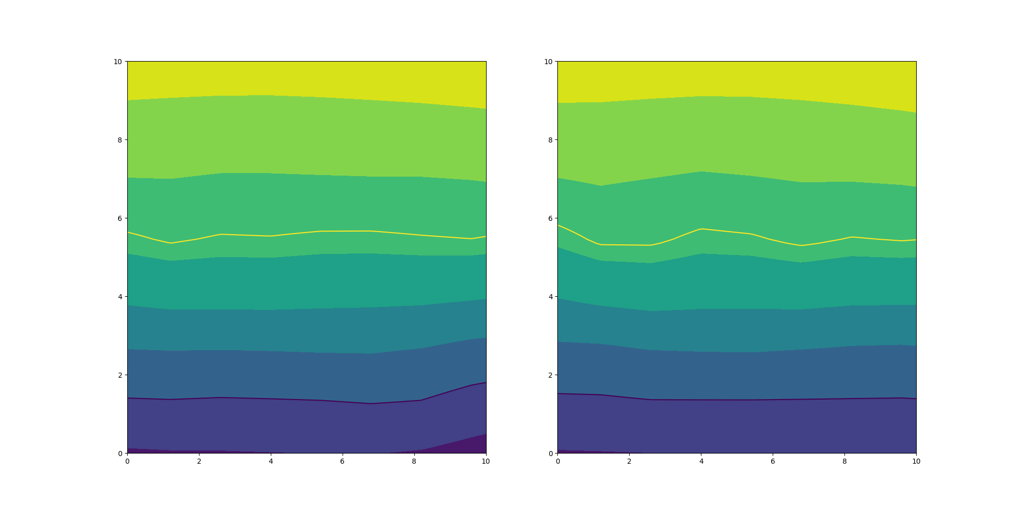
Visualising a 2-D section#
Geological feature can be evaluated:
* for the scalar field value at a location
* for the gradient of the scalar field at a location
To evaluate a model feature (scalar value or gradient) use the:
model.evaluate_feature_value(feature_name, locations) or
model.evaluate_feature_gradient(feature_name, locations)
Where the feature_name is the string naming the feature and locations is a numpy array of
xyz coordinates.
In the following example we will use matplotlib to visualise these results however, the next tutorial will show how to use the lavavu visualisation model.
import matplotlib.pyplot as plt

# X section
y = np.linspace(0, 10, 100)
z = np.linspace(0, 10, 100)

yy, zz = np.meshgrid(y, z)
xx = np.zeros_like(yy)
xx[:] = 5

vals = model.evaluate_feature_value(
    "conformable", np.array([xx.flatten(), yy.flatten(), zz.flatten()]).T
)
fig, ax = plt.subplots(1, 2, figsize=(20, 10))
ax[0].contourf(vals.reshape((100, 100)), extent=(0, 10, 0, 10))
ax[0].contour(vals.reshape((100, 100)), [0, 1], extent=(0, 10, 0, 10))

# Y section
x = np.linspace(0, 10, 100)
z = np.linspace(0, 10, 100)

xx, zz = np.meshgrid(x, z)
yy = np.zeros_like(xx)
yy[:] = 5

vals = model.evaluate_feature_value(
    "conformable", np.array([xx.flatten(), yy.flatten(), zz.flatten()]).T
)
ax[1].contourf(vals.reshape((100, 100)), extent=(0, 10, 0, 10))
ax[1].contour(vals.reshape((100, 100)), [0, 1], extent=(0, 10, 0, 10))

plt.show()

Total running time of the script: (0 minutes 0.853 seconds)