Implicit Geological Modelling#
Implicit geological modelling is an approach for representing objects in a geological model using mathematical function \(f(x,y,z)\) where the function returns the distance to the geological feature. Implicit modelling involves approximating the geometry of the geological object by using observations of the location and shape of the geological objects.
Building a basic implicit function#
For example, if we have a fault on a map. The geometry of this fault is defined by a trace on the map. If we want to approximate an implicit function that represents this geometry then we would need to find the function \(f(x,y,z)\) where \(f(x,y,z) = 0`\) at the observations of the fault trace. This function is under constrained and the best solution would be a function that is 0 everywhere. To further constrain this function we either need to add additional value constraints that are not 0 or a constraint to the gradient norm of the function. In a geological context, the gradient norm would be representative of the strike/dip of a geological object with some sense of younging (or a consistent direction for all observations).
import numpy as np
import pandas as pd
from LoopStructural.visualisation import Loop3DView
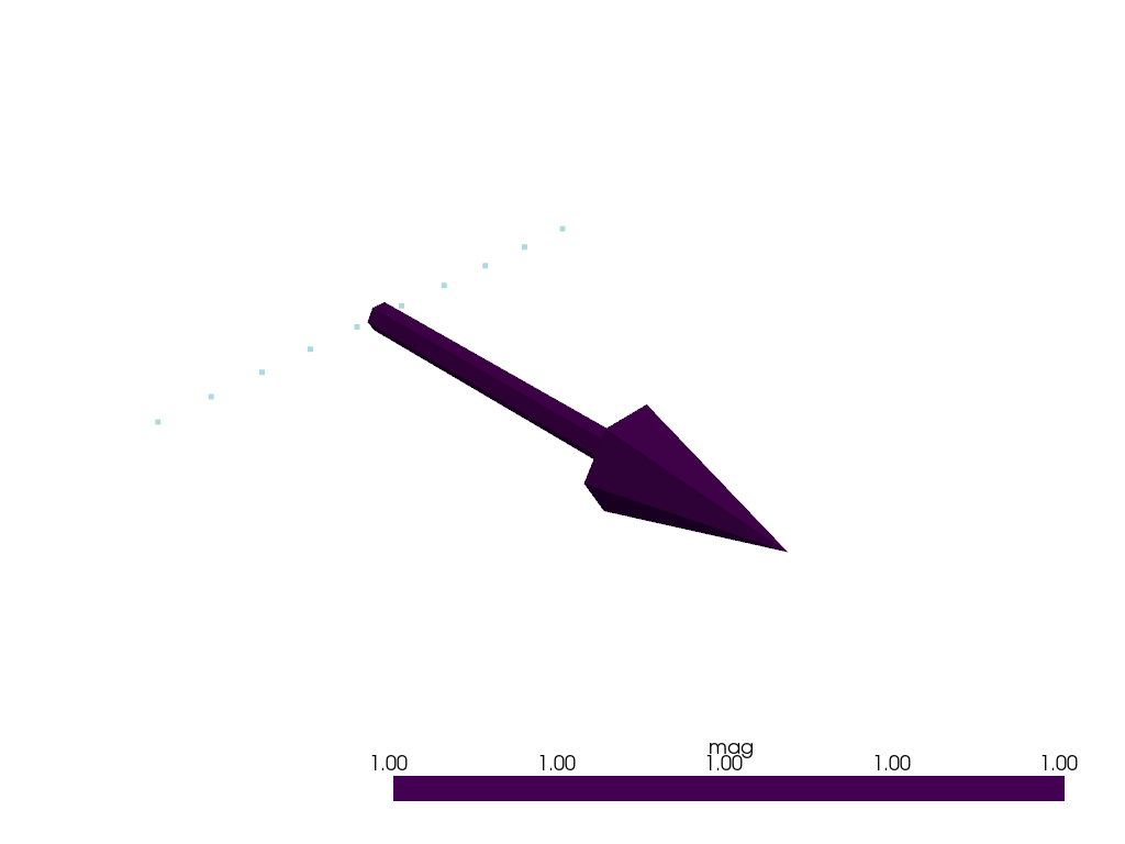
x = np.linspace(0, 1, 10)
y = np.zeros(10)
z = np.ones(10)
v = np.zeros(10)
data = pd.DataFrame({"X": x, "Y": y, "Z": z, "val": v})
vector = pd.DataFrame(
[[0.5, 0, 1.0, 0, 1, 0]], columns=["X", "Y", "Z", "nx", "ny", "nz"]
)
view = Loop3DView()
view.add_points(data[["X", "Y", "Z"]].values)
view.add_arrows(
vector[["X", "Y", "Z"]].values,
vector[["nx", "ny", "nz"]].values,
)
view.show()
To fit an implicit function using LoopStructural we can use the InterpolatorBuilder to create an interpolator that fits the value and orientation data as gradient norm constraints. The interpolator can be evaluated on a grid to visualise the geometry of the geological object.
import numpy as np
import pandas as pd
from LoopStructural import InterpolatorBuilder, BoundingBox
from LoopStructural.visualisation import Loop3DView

bounding_box = BoundingBox(np.array([-2, -2, -2]), np.array([2, 2, 2]))

interpolator = (
    InterpolatorBuilder(
        interpolatortype="FDI", nelements=1e4, bounding_box=bounding_box
    ).add_value_constraints(data.values)
    .add_normal_constraints(vector.values).setup_interpolator()
    .build()
)
mesh = bounding_box.structured_grid()
mesh.properties['val'] = interpolator.evaluate_value(mesh.nodes)
view = Loop3DView()
view.add_mesh(mesh.vtk())
view.show()
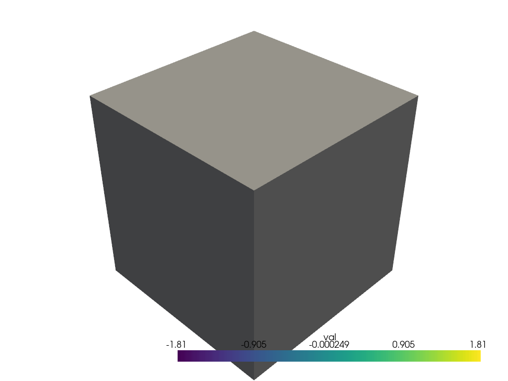
The resulting scalar field measures the distance to a reference horizon from -2 to 2.
We can extract an isosurface of the scalar field at 0 to visualise the geometry of the fault.
view = Loop3DView()
view.add_mesh(mesh.vtk().contour([0]))
view.add_points(data[["X", "Y", "Z"]].values)
view.add_arrows(
    vector[["X", "Y", "Z"]].values,
    vector[["nx", "ny", "nz"]].values,
)
view.show()
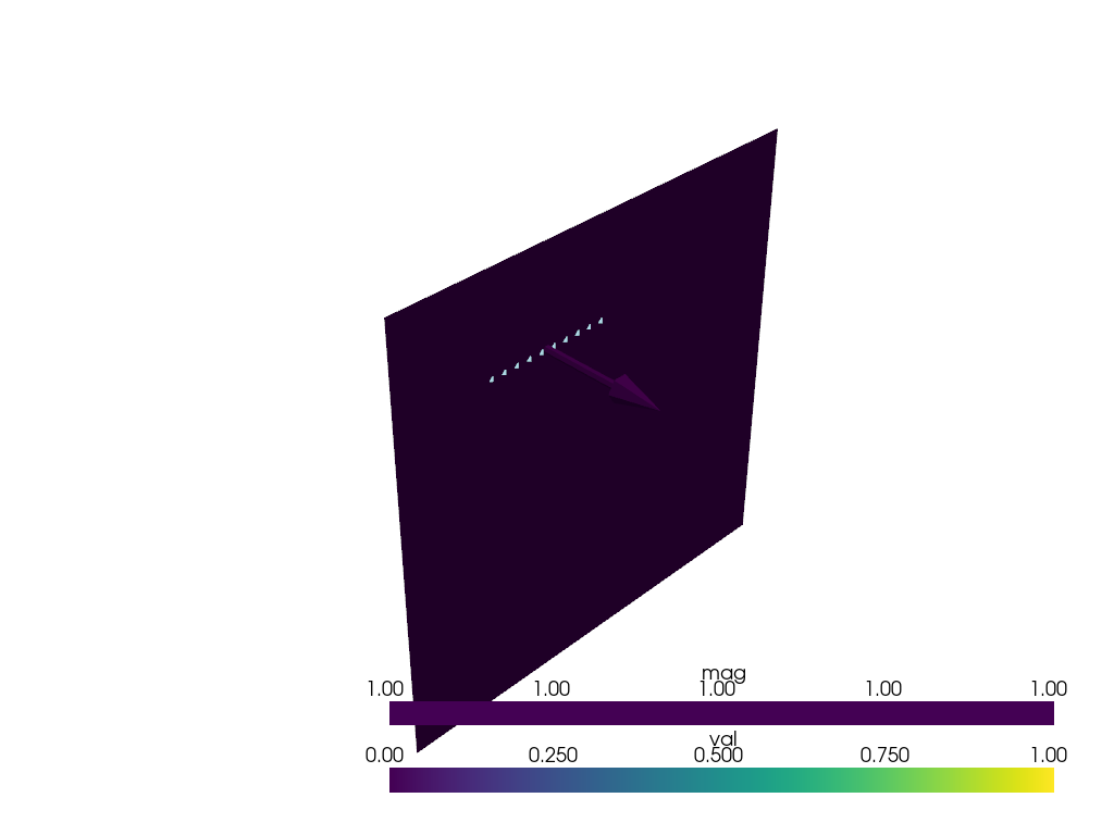
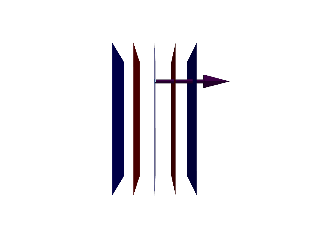
The resulting isosurface represents the geometry of the fault. The norm of the gradient of the scalar field controls how quickly we increase or decrease the scalar field value. For a single geological feature this is not particularly important but when we have multiple features represented by a single implicit function this can be important. Below shows the isovalues of -1,0,1 of the scalar field.
view = Loop3DView()
view.add_mesh(mesh.vtk().contour([-1, 0, 1]))
view.remove_scalar_bar()
view.add_points(data[["X", "Y", "Z"]].values)
view.add_arrows(
    vector[["X", "Y", "Z"]].values,
    vector[["nx", "ny", "nz"]].values,
)
view.remove_scalar_bar()
view.view_yz()
view.show()
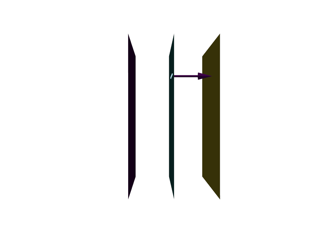
We can see that the length of the vector (unit vector) coincides with the distance between the two surfaces. If we were to change the length of the vector we would change the distance between the two surfaces.
vector[["nx", "ny", "nz"]] = vector[["nx", "ny", "nz"]]*2
bounding_box = BoundingBox(np.array([-2, -2, -2]), np.array([2, 2, 2]))

interpolator = (
    InterpolatorBuilder(
        interpolatortype="FDI", nelements=1e4, bounding_box=bounding_box
    ).add_value_constraints(data.values)
    .add_normal_constraints(vector.values).setup_interpolator()
    .build()
)
mesh2 = bounding_box.structured_grid()
mesh2.properties['val'] = interpolator.evaluate_value(mesh2.nodes)
view = Loop3DView()
view.add_mesh(mesh2.vtk().contour([-1, 0, 1]),color='red')
view.add_mesh(mesh.vtk().contour([-1, 0, 1]),color='blue')
view.add_points(data[["X", "Y", "Z"]].values)
view.add_arrows(
    vector[["X", "Y", "Z"]].values,
    vector[["nx", "ny", "nz"]].values,
)
view.remove_scalar_bar()
view.view_yz()
view.show()
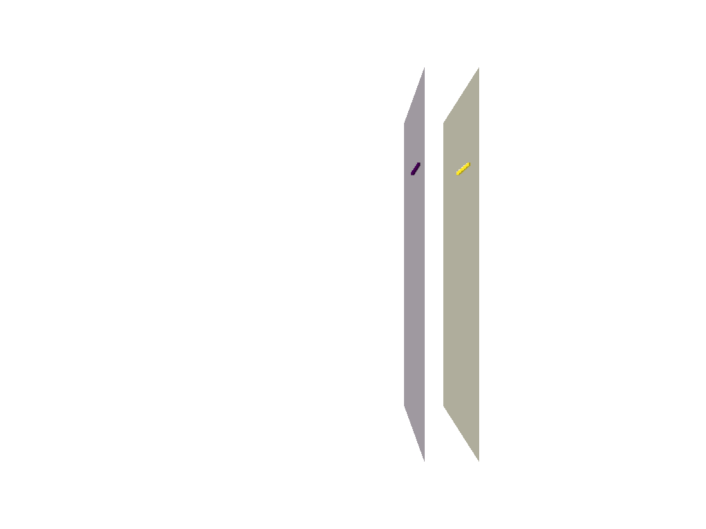
This time the vector is twice as long and the distance between the surfaces is half. This is because we have specified that the gradient of the scalar field has a magnitude of 2 which means that it grows twice as quickly.
Modelling with only value constraints#
An alternative approach for constraining the scalar field is to use only value constraints. This is useful when modelling a stratigraphic series where we may try to interpolate the distance to a contact and use the cummulative thickness between the stratigraphic units to constrain the value of the implicit function.
Following the example above we will use two lines of points with a value of 0 and 0.5 to represent two contacts between stratigraphic units.
import numpy as np
import pandas as pd
from LoopStructural import InterpolatorBuilder, BoundingBox
from LoopStructural.visualisation import Loop3DView

x = np.linspace(0, 1, 10)
y = np.zeros(10)
z = np.ones(10)
v = np.zeros(10)

data = pd.concat(
    [
        pd.DataFrame({"X": x, "Y": y, "Z": z, "val": v}),
        pd.DataFrame({"X": x, "Y": y + 0.5, "Z": z, "val": v + 0.5}),
    ]
)

bounding_box = BoundingBox(np.array([-2, -2, -2]), np.array([2, 2, 2]))

interpolator = (
    InterpolatorBuilder(
        interpolatortype="FDI", nelements=1e4, bounding_box=bounding_box
    )
    .add_value_constraints(data.values)
    .setup_interpolator()
    .build()
)
mesh = bounding_box.structured_grid()
mesh.properties["val"] = interpolator.evaluate_value(mesh.nodes)
view = Loop3DView()
view.add_mesh(mesh.vtk().contour([0, 0.5]), opacity=0.4)
view.remove_scalar_bar()
view.add_points(data[["X", "Y", "Z"]].values, scalars=data["val"].values)
view.remove_scalar_bar()

view.view_yz()
view.show()
We can see that the scalar field fits the value constraints and interpolates between the two surfaces. The scalar field value constraints can have a significant impact on the geometry of the implicit function, especially where the the geometry of the contacts outlies a structure (e.g. folded layers). Larger differences between the scalar field value effectively increase the magnitude of the implicit functions gradient norm.