Note
Go to the end to download the full example code.
4.a Building a model using the ProcessInputData#
There is a disconnect between the input data required by 3D modelling software and a geological map. In LoopStructural the geological model is a collection of implicit functions that can be mapped to the distribution of stratigraphic units and the location of fault surfaces. Each implicit function is approximated from the observations of the stratigraphy, this requires grouping conformable geological units together as a singla implicit function, mapping the different stratigraphic horizons to a value of the implicit function and determining the relationship with geological structures such as faults. In this tutorial the ProcessInputData class will be used to convert geologically meaningful datasets to input for LoopStructural. The ProcessInputData class uses: * stratigraphic contacts* stratigraphic orientations* stratigraphic thickness* stratigraphic order To build a model of stratigraphic horizons and:* fault locations* fault orientations * fault properties* fault edges To use incorporate faults into the geological model.
Imports#
from LoopStructural.modelling import ProcessInputData
from LoopStructural import GeologicalModel
from LoopStructural.visualisation import Loop3DView
from LoopStructural.datasets import load_geological_map_data

import matplotlib.pyplot as plt
Read stratigraphy from csv#
(
    contacts,
    stratigraphic_orientations,
    stratigraphic_thickness,
    stratigraphic_order,
    bbox,
    fault_locations,
    fault_orientations,
    fault_properties,
    fault_edges,
) = load_geological_map_data()

thicknesses = dict(
    zip(
        list(stratigraphic_thickness["name"]),
        list(stratigraphic_thickness["thickness"]),
    )
)
Stratigraphic Contacts#
contacts

fig, ax = plt.subplots(1)
ax.scatter(contacts["X"], contacts["Y"], c=contacts["name"].astype("category").cat.codes)
ax.set_title("Contact data")
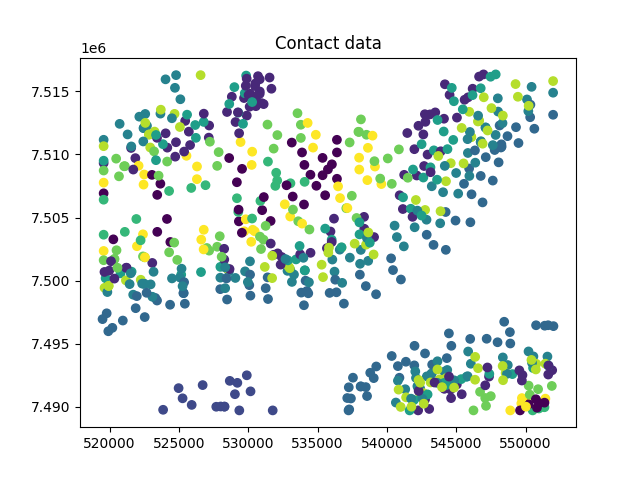
Text(0.5, 1.0, 'Contact data')
Stratigraphic orientations#
Stratigraphic orientations needs to have X, Y, Z and either azimuth and dip, dipdirection and dip, strike and dip (RH thumb rule) or the vector components of the normal vector (nx, ny, nz)
stratigraphic_orientations
Stratigraphic thickness#
Stratigraphic thickness should be a dictionary containing the unit name (which should be in the contacts table) and the corresponding thickness of this unit.
thicknesses
{'Mount_McRae_Shale_and_Mount_Sylvia_Formation': 224.5, 'Marra_Mamba_Iron_Formation': 152.0, 'Boolgeeda_Iron_Formation': 166.5, 'Woongarra_Rhyolite': 389.0, 'Jeerinah_Formation': 600.0, 'Brockman_Iron_Formation': 557.0, 'Wittenoom_Formation': 236.0, 'Weeli_Wolli_Formation': 241.5, 'Turee_Creek_Group': 162.0, 'Fortescue_Group': 236.0, 'Bunjinah_Formation': 236.0, 'Pyradie_Formation': 236.0}
Bounding box#
Origin - bottom left corner of the model # * Maximum - top right hand corner of the model
origin = bbox.loc["origin"].to_numpy()  # np.array(bbox[0].split(',')[1:],dtype=float)
maximum = bbox.loc["maximum"].to_numpy()  # np.array(bbox[1].split(',')[1:],dtype=float)

bbox
Stratigraphic column#
The order of stratrigraphic units is defined a list of tuples containing the name of the group and the order of units within the group. For example there are 7 units in the following example that form two groups.
# example nested list
[
    ("youngest_group", ["unit1", "unit2", "unit3", "unit4"]),
    ("older_group", ["unit5", "unit6", "unit7"]),
]

stratigraphic_order

order = [("supergroup_0", list(stratigraphic_order["unit name"]))]
Building a stratigraphic model#
A ProcessInputData onject can be built from these datasets using the argument names. A full list of possible arguments can be found in the documentation.
processor = ProcessInputData(
    contacts=contacts,
    contact_orientations=stratigraphic_orientations.rename({"formation": "name"}, axis=1),
    thicknesses=thicknesses,
    stratigraphic_order=order,
    origin=origin,
    maximum=maximum,
)
processor.foliation_properties["supergroup_0"] = {"regularisation": 1.0}
The process input data can be used to directly build a geological model
model = GeologicalModel.from_processor(processor)
model.update()
Or build directly from the dataframe and processor attributes.
model2 = GeologicalModel(processor.origin, processor.maximum)
model2.data = processor.data
model2.create_and_add_foliation("supergroup_0")
model2.update()
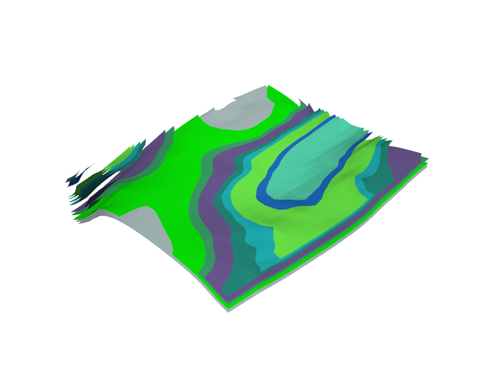
Visualising model#
view = Loop3DView(model)
view.plot_model_surfaces()
view.display()
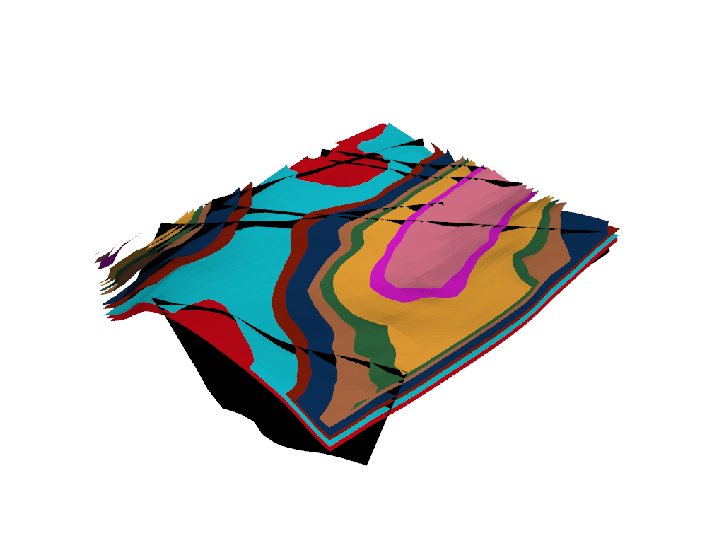
Adding faults#
fault_orientations


fault_edges


fault_properties

processor = ProcessInputData(
    contacts=contacts,
    contact_orientations=stratigraphic_orientations.rename({"formation": "name"}, axis=1),
    thicknesses=thicknesses,
    stratigraphic_order=order,
    origin=origin,
    maximum=maximum,
    fault_edges=fault_edges,
    fault_orientations=fault_orientations,
    fault_locations=fault_locations,
    fault_properties=fault_properties,
)
processor.foliation_properties['supergroup_0']['regularisation'] = 1.0
model = GeologicalModel.from_processor(processor)
model.update()

view = Loop3DView(model)
view.plot_model_surfaces()
view.display()
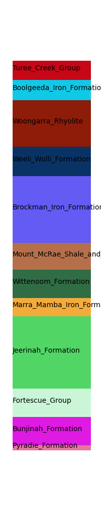
Visualise stratigraphic column ## ~~~~~~~~~~~~~~~~~~~~~~~~~~~~~
from LoopStructural.visualisation import StratigraphicColumnView

scv = StratigraphicColumnView(model)
scv.plot()
<Figure size 200x1000 with 1 Axes>
Total running time of the script: (0 minutes 16.735 seconds)