3b. Modelling a fault network in LoopStructural

Uses GeologicalModel, ProcessInputData and Loop3DView from LoopStructural library. Also using geopandas to read a shapefile, pandas, matplotlib and numpy.

import LoopStructural

LoopStructural.__version__

from LoopStructural import GeologicalModel
from LoopStructural.modelling import ProcessInputData
from LoopStructural.visualisation import Loop3DView
from LoopStructural.datasets import load_fault_trace
from LoopStructural.utils import rng
import pandas as pd
import matplotlib.pyplot as plt
import numpy as np

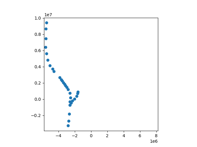
Read shapefile

Read the shapefile and create a point for each node of the line

fault_trace = load_fault_trace()
faults = []
for i in range(len(fault_trace)):
    for x, y in zip(fault_trace.loc[i, :].geometry.xy[0], fault_trace.loc[i, :].geometry.xy[1]):
        faults.append(
            [fault_trace.loc[i, "fault_name"], x, y, rng.random() * 0.4]
        )  # better results if points aren't from a single plane
df = pd.DataFrame(faults, columns=["fault_name", "X", "Y", "Z"])

fig, ax = plt.subplots()
ax.scatter(df["X"], df["Y"])
ax.axis("square")

scale = np.min([df["X"].max() - df["X"].min(), df["Y"].max() - df["Y"].min()])
df["X"] /= scale
df["Y"] /= scale

Orientation data

We can generate vertical dip data at the centre of the fault.

ori = []
for f in df["fault_name"].unique():
    centre = df.loc[df["fault_name"] == f, ["X", "Y", "Z"]].mean().to_numpy().tolist()
    tangent = (
        df.loc[df["fault_name"] == f, ["X", "Y", "Z"]].to_numpy()[0, :]
        - df.loc[df["fault_name"] == f, ["X", "Y", "Z"]].to_numpy()[-1, :]
    )
    norm = tangent / np.linalg.norm(tangent)
    norm = norm.dot(np.array([[0, -1, 0], [1, 0, 0], [0, 0, 0]]))
    ori.append([f, *centre, *norm])  # .extend(centre.extend(norm.tolist())))
# fault_orientations = pd.DataFrame([[
ori = pd.DataFrame(ori, columns=["fault_name", "X", "Y", "Z", "gx", "gy", "gz"])

Model extent

# Calculate the bounding box for the model using the extent of the shapefiles. We make the Z coordinate 10% of the maximum x/y length.

z = np.max([df["X"].max(), df["Y"].max()]) - np.min([df["X"].min(), df["Y"].min()])
z *= 0.2
origin = [df["X"].min() - z, df["Y"].min() - z, -z]
maximum = [df["X"].max() + z, df["Y"].max() + z, z]

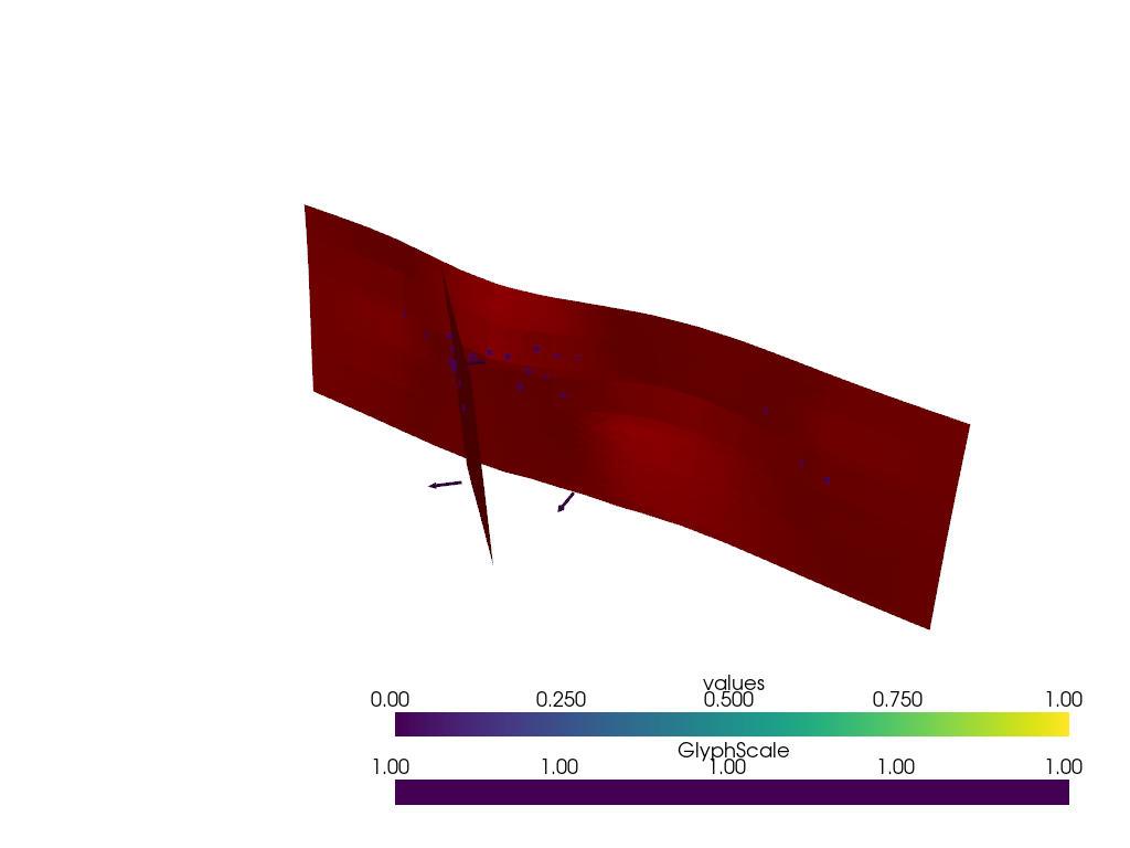
Modelling abutting faults

In this exampe we will use the same faults but specify the angle between the faults as \(40^\circ\) which will change the fault relationship to be abutting rather than splay.

processor = ProcessInputData(
    fault_orientations=ori,
    fault_locations=df,
    origin=origin,
    maximum=maximum,
    fault_edges=[("fault_2", "fault_1")],
    fault_edge_properties=[{"angle": 40}],
)

model = GeologicalModel.from_processor(processor)

view = Loop3DView(model)
for f in model.faults:
    view.plot_surface(f, value=[0])  #
    view.plot_data(f[0])

view.display()