Note
Go to the end to download the full example code.
2a. Modelling folds#
This tutorial will show how Loop Structural improves the modelling of folds by using an accurate parameterization of folds geometry. This will be done by: 1. Modelling folded surfaces without structural geology, i.e. using only data points and adjusting the scalar fields to those points. 2. Modelling folds using structural geology, which includes: * Description of local fold frame and rotation angles calculation * Construction of folded foliations using fold geostatistics inside the fold frame coordinate system
Imports#
from LoopStructural import GeologicalModel
from LoopStructural.datasets import load_noddy_single_fold
from LoopStructural.visualisation import Loop3DView, RotationAnglePlotter
import pandas as pd
Structural geology of folds#
Folds are one of the most common features found in deformed rocks and are defined by the location of higher curvature. The geometry of the folded surface can be characterised by three geometrical elements:
the fold hinge is the point of maximum curvature along folded surface
the axial surface is a surfaces that passes through all curvature points in all folded foliations
the fold axis is the intersection of the folded foliation and the axial surface
Modelling folded surfaces using standard implicit algorithms is challenging because the implicit modelling methods are generally trying to minimise the resulting curvature of the surface. To model folded surfaces the geologist will need to characterise the geometry of the folded surface in high detail.
Modelling folded surfaces without structural geology#
In the following section we will attempt to model a synthetic fold shape that is defined by a sinusoidal folded surface. For simplicity we will consider the fold as cylindrical and therefore only consider the fold in a 2D plane. The data set has been sampled from a model generated using Noddy and represents a fold with a wavelength of ~10km and amplitude of ~2km.
The orientation of the structure has been sampled within the model volume (10km,7km,5km) at 500m intervals.
The aim of this exercise is to investigate how standard implicit modelling techniques are fundamentally limited when trying to model folded surfaces.
Load data from sample datasets
Visualise data
Look at varying degrees of sampling e.g. 200 points, 100 points, 10 points.
Look at using data points ONLY from a map surface
Modelling folded surfaces using loop structural#
# load the sample data
data, boundary_points = load_noddy_single_fold()
data.head()
The input dataset was generated using Noddy by sampling the orientation
of a structure on a regular grid. We have loaded it into a pandas
DataFrame, this is basically an excel spreadsheet for python. Above are
the first 5 rows of the dataset and as we can see it is regularly
sampled with data points being sampled regularly along the \(z\),
\(y\) and \(x\) axes. In order to avoid artefacts due to the
sampling errors we will shuffle the data. We can do this using the
random column in the DataFrame (ensuring everyone has the same
data).
data = data.sort_values(
    "random"
)  # sort the data by a random int then we can select N random points
data.head()
The data points are now randomly ordered and can now be subsampled by choosing the first N samples from the dataframe
data[:100]
returns the first 100 data points from the array
Testing data density#
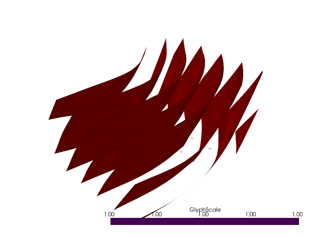
Use the toggle bar to change the amount of data used by the interpolation algorithm.
How does the shape of the fold change as we remove data points?
Now what happens if we only consider data from the map view?
HINT you can view the strike and dip data by unchecking the scalar field box.
The black arrows are the normal vector to the folded surface
npoints = 20
model = GeologicalModel(boundary_points[0, :], boundary_points[1, :])
model.set_model_data(data[:npoints])
stratigraphy = model.create_and_add_foliation(
    "s0", interpolatortype="PLI", nelements=5000, buffer=0.3, cgw=0.1
)  # .2)
viewer = Loop3DView(model, background="white")
# viewer.add_scalar_field(model.bounding_box,(38,55,30),
#                       'box',
#                      paint_with=stratigraphy,
#                      cmap='prism')
viewer.plot_data(stratigraphy)
viewer.plot_surface(stratigraphy, value=10)
viewer.show()

Modelling folds using structural geology#
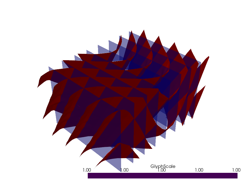
The following section will describe how the fold axis, fold axial surface and fold vergence can be used to help constrain the shape of the folded surface. To do this we need to build a fold frame which is curvilinear coordinate system based around the fold axis and the fold axial surface.
There are three coordinates to the fold frame: * coordinate 0 is the axial surface of the fold and is parallel to the axial foliation * coordinate 1 is the fold axis direction field and is orthogonal to the axial foliation * coordinate 2 is orthogonal to both the fold axis direction field and axial foliation and is roughly parallel to the extension direction of the fold
Three direction vectors are defined by the normalised gradient of these fields: * \(e_0\) - red * \(e_1\) - green * \(e_2\) - blue
The orientation of the folded foliation can be defined by rotating \(e_1\) around \(e_0\) by the fold axis rotation angle \(\alpha_P\) to give the orientation of the fold axis. The orientation of the folded foliation can then be defined by rotating the plane defined by the fold axis and \(e_0\) around the fold axis by the fold limb rotation angle \(\alpha_L\).
Calculating the fold rotation angles#
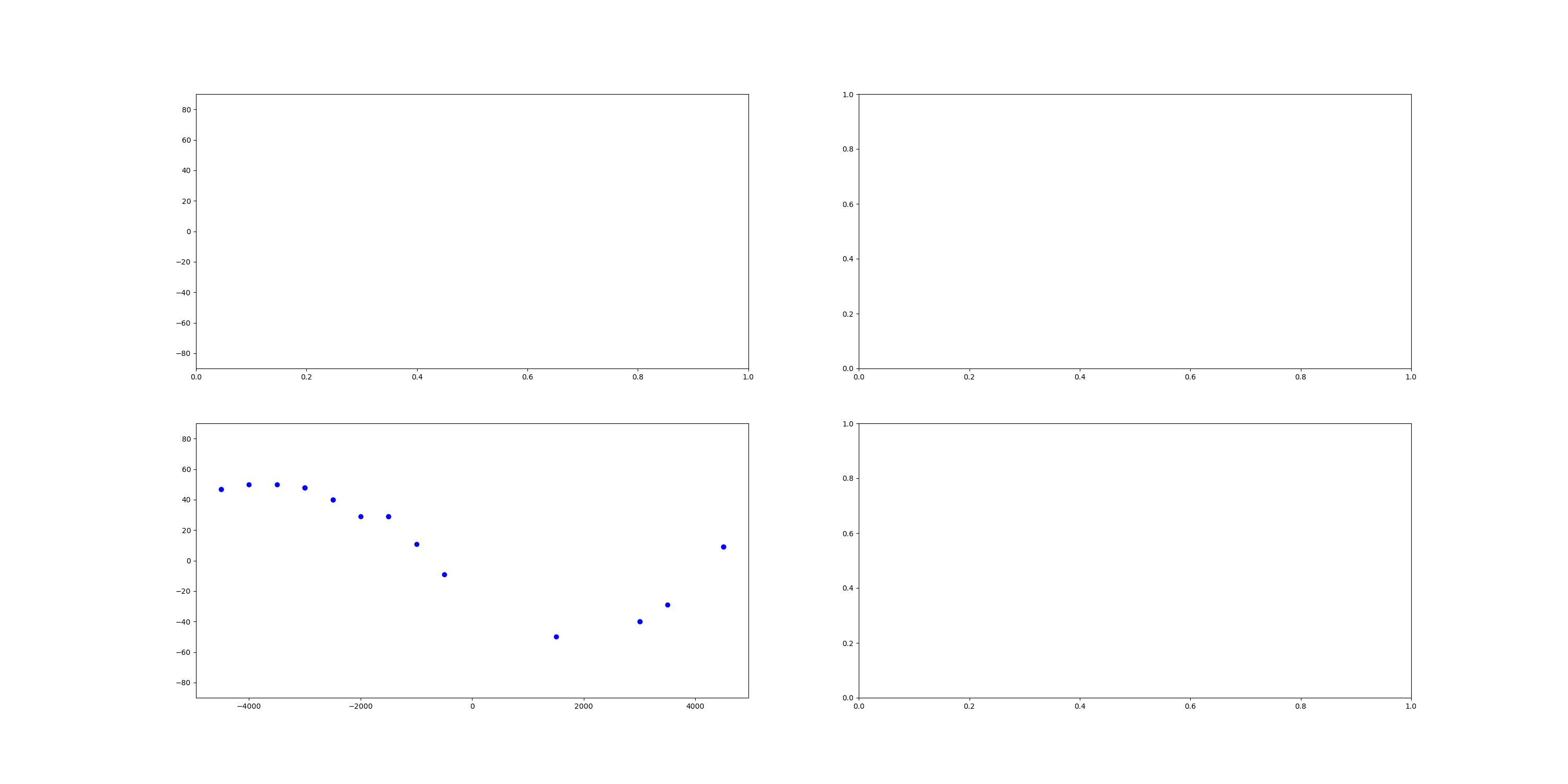
The rotation angles can be calculated for observations of the folded foliation and assocaited lineations. For example, the fold axis rotation angle is found by calculating the angle between the gradient of the fold axis direction field and the intersection lineations shown in A). The fold limb rotation angle is found by finding the the angle to rotate the folded foliation to be parallel to the plane of the axial foliation shown in B and C. The wavelength can be specified by the user or in some cases estimated from the s-variogram of the fold frame coordinate system.
mdata = pd.concat([data[:npoints], data[data["feature_name"] == "s1"]])
model = GeologicalModel(boundary_points[0, :], boundary_points[1, :])
model.set_model_data(mdata)
fold_frame = model.create_and_add_fold_frame(
    "s1",
    interpolatortype="PLI",
    nelements=10000,
    buffer=0.5,
)
stratigraphy = model.create_and_add_folded_foliation(
    "s0",
    fold_frame=fold_frame,
    nelements=10000,
    fold_axis=[-6.51626577e-06, -5.00013645e-01, -8.66017526e-01],
    limb_wl=12000,
    buffer=0.5,
)
viewer = Loop3DView(model, background="white")
# viewer.add_scalar_field(model.bounding_box,(38,55,30),
#                       'box',
#                      paint_with=stratigraphy,
#                      cmap='prism')
viewer.plot_surface(
    fold_frame[0],
    value=10,
    colour="blue",
    #                       isovalue=0.4,
    opacity=0.5,
)
viewer.plot_data(stratigraphy)
# viewer.add_isosurface(fold_frame[1],colour='green',alpha=0.5)
# viewer.add_vector_field(fold_frame[0],locations=fold_frame[0].get_interpolator().support.barycentre)
# viewer.add_data(fold_frame[1])

# viewer.add_data(stratigraphy)
viewer.plot_surface(stratigraphy, value=10)
viewer.show()

Plotting the fold rotation angles#
rotation_plots = RotationAnglePlotter(stratigraphy)
rotation_plots.add_fold_limb_data()
rotation_plots.add_fold_limb_curve()
rotation_plots.add_limb_svariogram()
# plt.plot(stratigraphy.builder.fold.fold_limb_rotation.fold_frame_coordinate,stratigraphy['limb_rotation'],'bo')
# x = np.linspace(fold_frame[0].min(),fold_frame[0].max(),100)
# plt.plot(x,stratigraphy['fold'].fold_limb_rotation(x),'r--')
rotation_plots.fig.show()

Total running time of the script: (0 minutes 5.870 seconds)